
Bayes from Scratch, Part 2: Bayesian Regression using Grid Search
This is Part 2 in the Bayes from Scratch series. Read Part 1 - Bayesian Grid Mean here.
In Part 1 I wanted to understand how Bayes Theorem could be used to compute the mean for a single variable without using MCMC, instead I used grid search. A brute force method that computes the posterior for a grid of every combination of parameters within some range.
Miles per Gallon by Engine Displacement
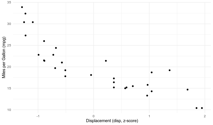
In Part 2 I'm going to try a regression. We just need to add one new parameter, and a structural equation. Miles-per-gallon mpg is distributed by a normal distribution with mean m and standard deviation s. The mean m is determined by the equation $m = \beta \cdot \text{disp} + \alpha$. The engine displacement variable is centered at the mean, so when disp is 0 the alpha parameter should represent the expected mpg for the average vehicle.
$$
mpg \sim Normal(m, s) \\
m = \beta \cdot \text{disp} + \alpha \\
\beta \sim Normal(0,2) \\
\alpha \sim Normal(18, 3) \\
s \sim Uniform(0, 20)
$$
Estimating Parameters using Grid Search
When I first attempted this, I had two predictors in the model (thus 4 parameters), for, you know, fun. This was a mistake. I was quickly reminded the curse of dimensionality. I pared it back to one new parameter. My laptop, with 16 GB of ram, can't actually compute a grid with N = 200.
N <- 200
g <- expand_grid(alpha = seq(1, 100, length.out = N)
                 , beta = seq(-10, 10, length.out = N)
                 , s = seq(0.1,20, length.out = N))
One of the problems with grid searches is you have to specify the bounds the grid a priori. Looking at the plot it's easy to see the slope will be negative, and we already know the mean value of mpg is somewhere between 15 and 25.
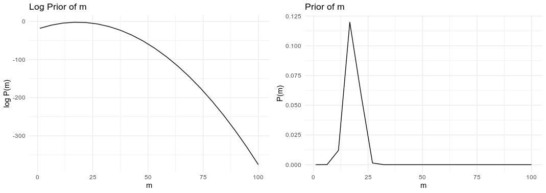
Priors: Advantages of Log Probabilities
The priors are pretty simple. The big difference between this run and the previous is that I'm going to be computing log probabilities. There are two great benefits to using log probabilities 1) floating point values can actually store log probabilities, and 2) we can take advantage of the Product Rule for Logarithms.
mpg_alpha_prior <- dnorm(g$alpha, mean = 18, sd = 3, log = TRUE)
mpg_s_prior <- dunif(g$s, min = 0, max = 20, log = TRUE)
mpg_beta_prior <- dnorm(g$beta, mean = 0, sd = 2, log = TRUE)
Some of the priors or posterior values in raw probabilities will be teeny tiny - very close to zero. Some of the values can be $10^{-100}$. This can be a real problem for floating point computation.
The second advantage is the product rule of logarithms. The sum of two logarithms is equal to the logarithm of a product. Bayes Theorem and probability theory relies the product of probabilities in many places, and by using the log probability we can sum the values instead.
$$
\log_{a} xy = \log_{a} x + \log_{a} y
$$
Estimating the Likelihood
The most computationally difficult part is computing the likelihood.
mm <- cbind(1, dcars$disp) # the model matrix
mpg_log_likelihood <- apply(g, 1, FUN = function(r) {
  params <- as.numeric(r[c('alpha', 'beta')])
  m <- as.numeric(mm %*% params)
  sum(dnorm(mtcars$mpg, mean = m,
            sd = as.numeric(r['s']), log = TRUE))
})
The g data frame has all the grid parameter values. I computed the likelihood at each combination of parameters on the grid. First we compute the value of the linear model using matrix multiplication: m <- as.numeric(mm %*% params) The matrix mm is the design matrix with a column of the data for the engine displacement, disp, and a column of 1's for the intercept. Then, using the logarithm product rule, I compute the likelihood for that combination of parameters: sum(dnorm(mtcars$mpg, mean = m, sd = as.numeric(r['s']), log = TRUE)).
Computing the Posterior
Then computing the posterior is pretty simple - the likelihood times the prior. Or in our case - the log likelihood plus the log prior. The raw posterior probability can be computed and normalized after computing the log posterior.
d <- g %>%
  mutate(mpg_ll = mpg_log_likelihood) %>%
  mutate(post = exp(mpg_log_post) / sum(exp(mpg_log_post)))
Posterior Checks
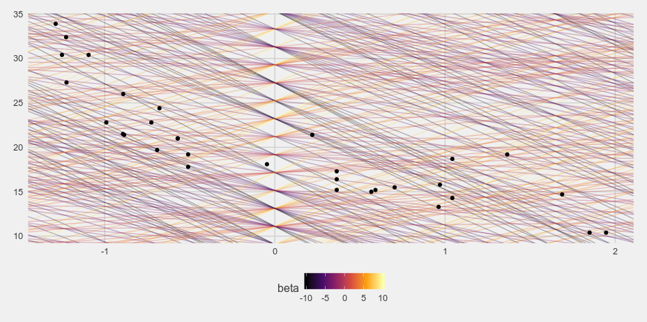
Let's see if this posterior makes sense. If we just randomly sample 1000 lines from the grid data frame and plot the different lines on a plot of the data we get something like this.
i <- sample(1:nrow(d), size = 1000, replace = TRUE)
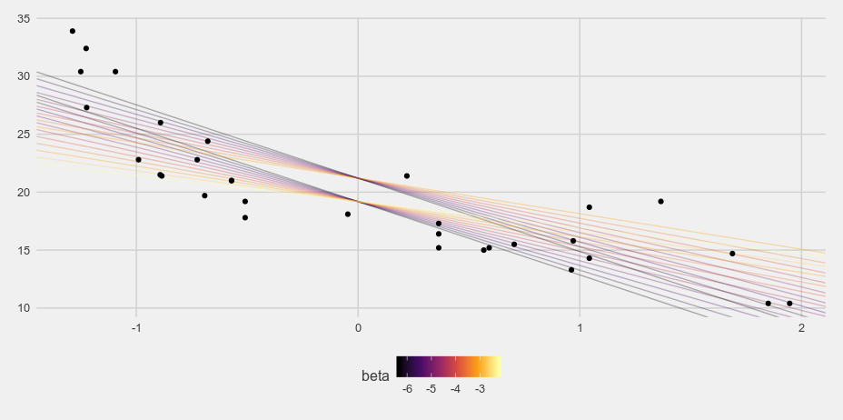
And when I weight the grid samples based on the posterior probability we get something much more reasonable:
i <- sample(1:nrow(d), size = 1000, prob = d$post, replace = TRUE)
# i <- sample(1:nrow(d), size = 1000, replace = TRUE)
ggplot() +
  geom_abline(data = d[i,], aes(slope = beta, intercept = alpha, color = beta),
              alpha = 0.3) +
  scale_color_viridis_c(option = 'B') +
  geom_point(data = dcars, aes(x = disp, y = mpg), ) +
  coord_cartesian(xlim = c(min(dcars$disp), max(dcars$disp))) +
  theme_fivethirtyeight()
Thoughts
My first thought - hey, this works! My second thought - this is incredibly imprecise and computationally expensive! I did the last few plots on my laptop, so I had to reduce the grid size dramatically compared to my beefy desktop machine. This is a really simple regression and the thought that it can't be computed on a relatively powerful laptop is a good indication that this approach is a bad choice.
But it shows that using Bayes Theorem to estimate models can be done simply - even if it is expensive. When you learn Bayesian statistics there is often so much tied up in trying to understand MCMC. This approach ignores MCMC entirely. Soon though I will write MCMC from scratch as well and pick it apart.